ScanImage® Coordinate Systems

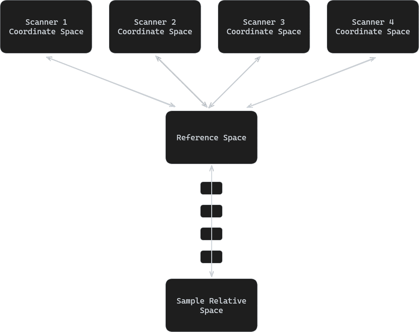
Each ScanImage® scanner (ResScan / LinScan) uses its own Scanner coordinate system to allow for different field of views accommodating for minor misalignments in the optical setup. Coordinates wrapped in this coordinate system can easily be transformed to the common reference space. The scanner, reference, and sample relative coordinate spaces are all used in the ScanImage® API and GUIs exposed to the user.

Scanner Coordinates

Each configured imaging scanner has its own Scanner Coordinate system.

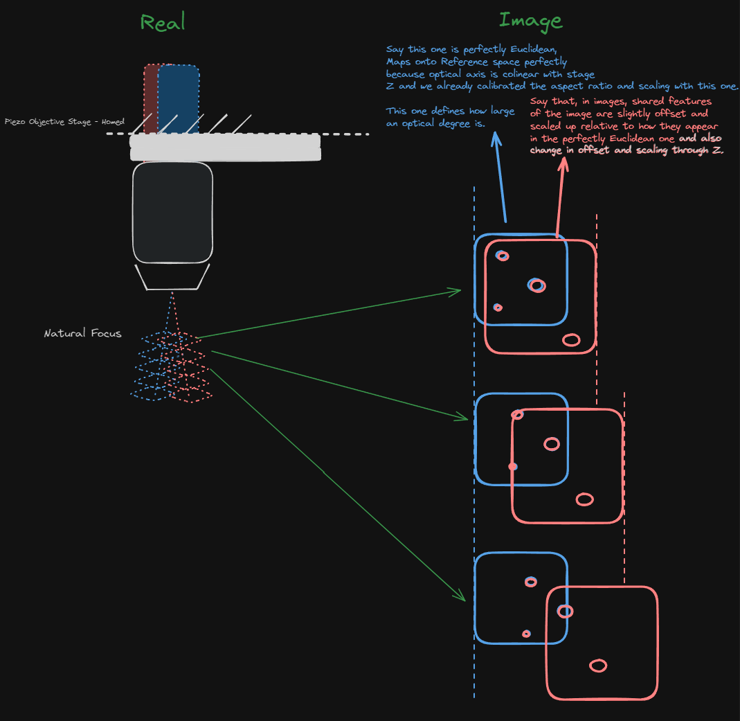
This coordinate system is scaled in optical degrees in X and Y as they are defined by the imaging scanner’s X and Y, and microns in Z as they are defined by its fastZ. Its origin is coincident with the reference coordinate system origin. The angle of the X, Y, and Z axes are such that they are parallel to the actual scanner X, scanner Y, and fastZ axes.

The optical system may be actualized with imperfections. The scaling of each axis is dependent on the paired X, Y, and Z scanners’ scaling factors set in resource configuration, and variation from actuators specs from the datasheet can lead to disagreement between axes in scaling. Configured scanners’ actuation at a minimum needs to be calibrated within or without scanimage to have linear control of position for galvanometer or fastZ devices, or linear control of resonant scanner amplitude.

Tip

Ideally, 1 optical degree in X is also 1 optical degree in Y in image space.

It is best to resolve this by configuring the scanners correctly from resource configuration.

Furthermore, the actual scanner X, Y, and fastZ axes may not be parallel to the ideal X, Y, and Z axes due to system misalignment.

Reference Coordinates

There are two things ScanImage can do to help with this variation of scanner axes orientation:

represent image data correctly in the reference coordinate space,
Alter scanning to actually scan as defined in the reference coordinate space accounting for imperfections.

For non-galvo-galvo scanning modalities, we can only represent images in as spatially correct a way as possible in the reference space. In other words, Resonant scanners imaging/stimuli/analysis ROIs are defined in scanner space and get mapped back to reference space to be displayed with any distortions found during the scannerToReference Alignment.

For galvo-galvo scanning, we are able to alter scanning to account for imperfections. In other words, Linear scanners’ imaging/stimuli/analysis ROIs are defined in reference space and then mapped back into the appropriate scanner space to control the scanner hardware.

Such graphics which are plotted in either reference space or scanner space based on selected imaging scanner are: - Default Imaging ROI - MROI Group ROIs - Stim ROIs - Scanfield power boxes - Integration ROIs - Quick Analysis ROIs - FOV and park position

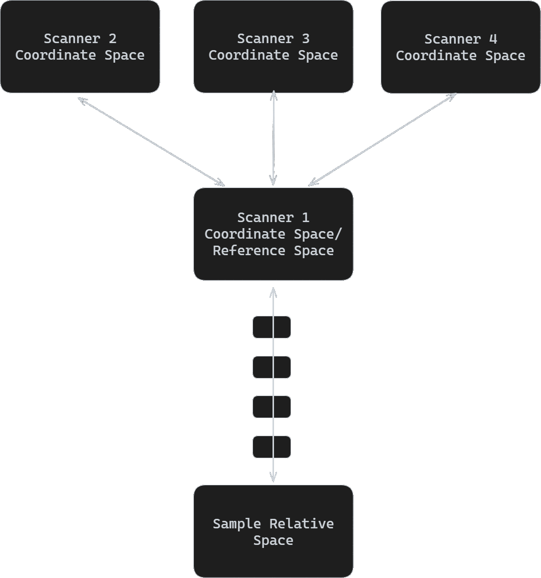
The reference space can be treated in one of two ways. It can be treated as an ideal space, or it can be treated as being identical to a primary scanner’s scanner space.

The ideal space has a 1:1 aspect ratio in XY with orthogonal XYZ axes. The scaling of the axes are optical degrees for X and Y, and microns for Z. Its origin follows the ideal focal point as though the optical system is free of imperfections like pupil shift and misalignment of scanner axes of rotation at the zero position of the X, Y, and fastZ scanners. The rotation is such that Z is parallel to the optical axis, and X is parallel to the ideal scanner X, with all axes orthogonal to one another.

Regardless of which way the reference space is treated, it is the common coordinate space.

Ideal Reference Space	Reference Space identical to Primary Scanner Space

The scanner spaces are mapped into a common reference space via affine transformation lookup table by Z (for flexible 3D characterization) determined during the scannerToReference Alignment.

../_images/CoordinateSystemsAccountForMisalignment.png

Since the origin follows the ideal focal point, items defined in the reference coordinate space move with a motorized stage such that they remain in their position relative to the idealized scannable volume under the objective.

Items plotted directly in this coordinate space are items that are capable of being scanned in this idealized space. Galvo-Galvo scanners can be fed scan patterns that counteract the misalignment of their imaging systems, and so if the imaging scanner is Galvo-Galvo, then graphics will be plotted in this space.

zRef = 20; %Reference space Z where the 2D affine should be taken
scannerToRef_ResScan = hSI.hResScan.hCSZAffineLut.toParentLutEntries.makeZAffines(zRef) % affine transformation for ResScan
scannerToRef_LinScan = hSI.hLinScan.hCSZAffineLut.toParentLutEntries.makeZAffines(zRef) % affine transformation for LinScan

Attention

The scannerToReference alignment tool is only available in Premium ScanImage.

Sample Relative Coordinate System

This coordinate system, when calibrated, is scaled in microns in X,Y, and Z with an origin that is stationary in space until arbitrarily placed by the user and a rotation that can be arbitrary with a session-session alignment or defining stage rotation, though it would otherwise remain with it’s X-axis parallel to the ideal scanner X with X, Y, and Z axes orthogonal.

Items plotted directly in this coordinate space are:

Tiles
Cycles
Pinned images
Annotations
Sample Power Boxes

for more information, see Sample Coordinate System

Scanfields, ROIs, ROI Groups

Scanfields

A scanfield is the 2D cross section of a ROI at a particular z plane. The discrete set of user defined scanfields defines the volumetric shape of the ROI.

Each scanfield is defined by the following set of properties:

centerXY: [x,y] coordinates of the scanfield in optical degrees in the coordinate system in which it is defined
sizeXY: [width, height] size of the scanfield in optical degrees in the coordinate system in which it is defined
pixelResolutionXY: pixels per line, number of lines
rotationDegrees: rotation of scanfield in degrees

ROIs

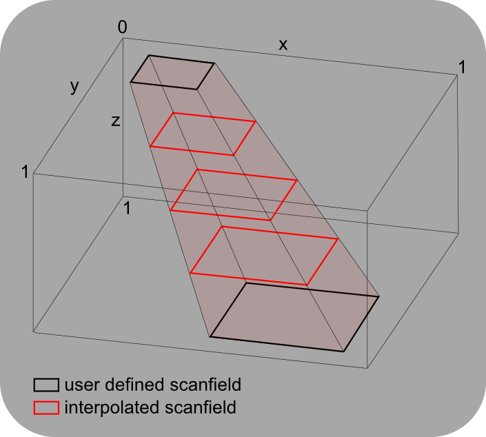
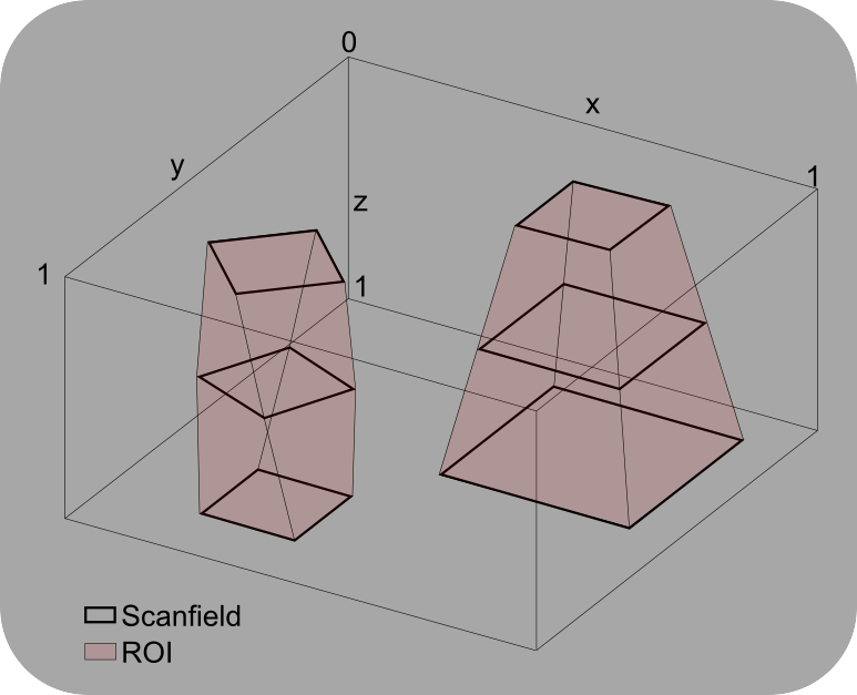
A ROI is a three dimensional volume defined by a set of one or more scanfields, each at a unique z-level. A ROI which contains only one scanfield stretches from z = -inf..inf. To limit the z extent of the ROI, define at least two second scanfields. Each scanfield is a control point in the shape of the 3D volume. Between control points, scanfields are interpolated. Alternatively, a ROI can exist only at discrete z planes only where scanfields are defined.

Note

The scanfields that you add to a ROI do not specify the z planes that will actually be imaged when you start an acquisition. The scanfields are only defining the shape of the 3D volume. The z planes to be imaged are set up through the FastZ GUI. For each z plane to be imaged, ScanImage® will look at the current ROI group to determine what ROIs exist at that z plane and extract the scanfield to be imaged.

Ex: In the example ROI on the left, scanfields are are defined at z planes of 0 and 10. For this example, suppose the user sets up a fast Z for 4 slices, 4 steps (microns) per slice. The actual z planes that will be imaged would be 0, 4, 8, and 12. The user defined scanfield 1 would be imaged at z plane 0, while interpolated scanfields between 0 and 10 would be imaged at z of 4 and 8. Nothing would be imaged at z of 12 because the ROI only exists between the top and bottom scanfields.

../_images/mROI%2BInterpolation.png — ROIs

x

y

width

height

z

scanfield 1

1

1

2

2

0

scanfield 2

5

5

4

4

10

A ROI consisting of two user defined scanfields at z=0 and z=10. If needed, scanfields are linearly interpolated for different values of z (red rectangles).

ROI Group

A collection of ROIs forms a ROI Group. During a volume acquisition, ScanImage® queries the ROI group to return the scanfields at a particular z plane. ScanImage® acquires images for each of the scanfields before moving on to the next z plane.

	x	y	width	height	z
scanfield 1	1	1	2	2	0
scanfield 2	5	5	4	4	10