Photon Counting
ScanImage® includes a photon counting module, which uses a fast acquisition sampling rate (>1GHz) to directly sample the output of the transimpedance amplifier. ScanImage® analyzes the voltage signal and performs a peak detection on the signal to count photons in real time. By synchronizing the fast digitizer to the sample clock, time correlated photon counting is supported. This allows ScanImage® to bin detected photons into virtual output channels depending on their arrival time.
The acquisition DAQ can be operated in photo current integration mode and photon counting simultaneously for each of the physical high speed analog input ports. This allows display of each to get a direct comparison between the two modes. It is possible to use photon integration for bright regions and photon counting for photon limited regions in the sample. This maximizes the dynamic range of the microscope, and provides an effective means of noise suppression in the low signal regions.
Note
Photon counting is most useful for photon limited experiments. This means that less than 1 or less photons are expected to arrive at the PMT per laser pulse. In this regime, photon peaks are clearly separated in the signal. Once the photon rate rises, photon responses start to overlap and the photon discrimination will count multiple photons as a single event. At this point it is advised to switch to photo current integration mode.
Photon counting uses different GUIs depending on choice of DAQ hardware. Select the page appropriate to your microscope to continue:
With a sampling rate of 2.0 GHz to 2.7 GHz, the vDAQ-HS can record at sub nanosecond time resolution. The signal conditioning controls created exclusively for the vDAQ can bin photons collected with this high resolution into any of 32 virtual channels based on user defined temporal windows.
Hardware Setup
High Speed vDAQ
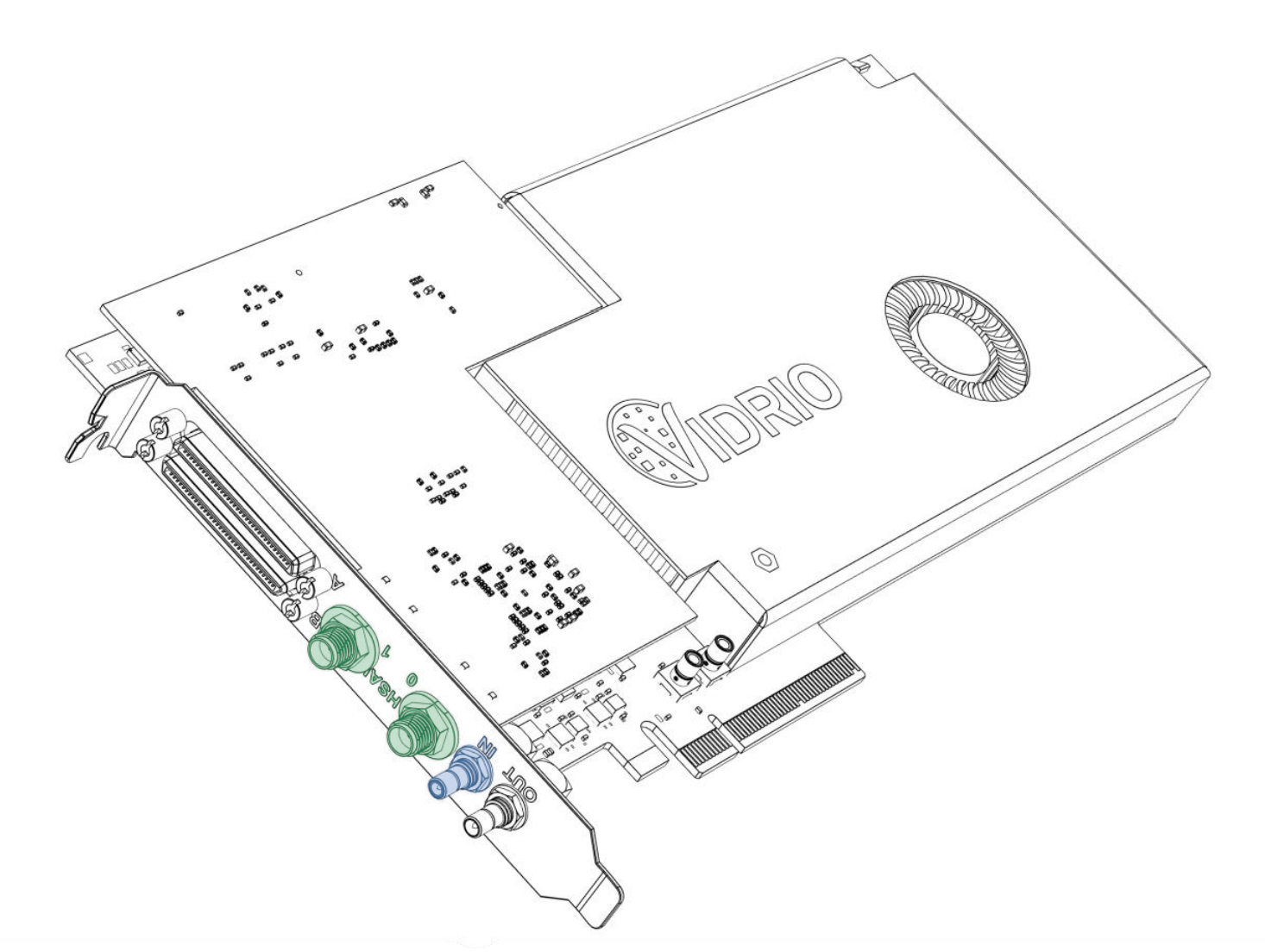
Connect amplified PMT signals to HSAI inputs highlighted green
(optionally) Connect a laser clock (62.5MHz-84.375MHz) to IN highlighted blue
The following hardware is used:
(optional) A fast transimpedance amplifier (bandwidth >80MHz) (such as the Femto DHPCA-100)
Note
In some instances, the fastest bandwidth signal is acquired without without a transimpedance amplifier.
(optional) For time correlated photon counting with a laser rep rate less than 1 MHz, a clock multiplier board such as the AD9516-0 is required
The high speed vDAQ is installed as is described in page vDAQ Installation.
Connect each Photomultiplier Tube (PMT) to the input of a separate high bandwidth transimpedance amplifier (TIA) and connect the the output of each TIA to the high speed analog inputs (HSAI) of the vDAQ. Alternatively, the output of the photomultiplier tube can be fed directly into a high speed analog input of the high speed vDAQ. The ports are enumerated 0 and 1 on the vDAQ card’s PCIe bracket. Each are SMA male connectors; the signal cable from the source to the HSAI ports may need to be adapted from a different style connector.
Software Tutorial
Here, simple photon counting, virtual channels, and time correlated photon counting will be shown. Each topic builds from the previous.
Photon Counting
First, photon counting without synchronizing to the laser clock will be shown, and then time correlated photon counting.
Photon Counting is managed through the Signal Conditioning Tab in the Auxiliary Panel, which is summoned from View>Auxiliary Panel>Signal Conditioning Tab. It is only available when the currently selected imaging system (as selected from the configuration window) is a vDAQ Scan System.
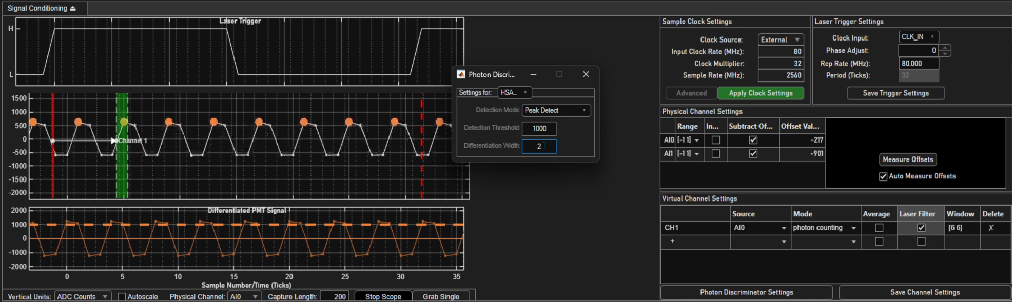
Bring up the Signal Conditioning Controls tab. First, notice the Signal Scope panel at the Left. The PMT signal can be monitored continuously,
or a specified Capture Length can be grabbed.
After preparing a sample where signal-to-noise ratio will be expected to be low and focusing at an appropriate depth,
leave the acquisition in a Focus state and press the Grab Single button in the Signal Conditioning tab under the plot axes.
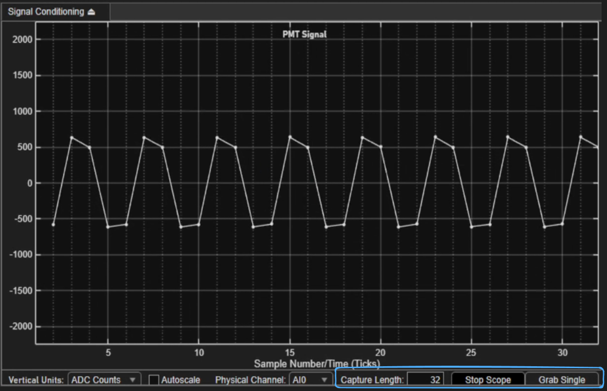
This will populate the PMT Signal graph with data. From this data, decisions can be made on settings such as tolerances required for a peak to be
counted as a photon. One can zoom in temporally by scrolling with the mouse wheel, or one can decrease the number of samples per grab, and do another grab.
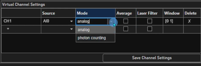
the Virtual Channel Settings contains a table with a row per virtual channel. In the Mode column (column 3) of this table, the integration (analog) or photon counting data pipeline
can be selected for each of the virtual channels.
The settings for determining how the photons are counted can be adjusted now.
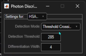
Under the Threshold Crossing detection mode, any crossing of the threshold from below to above is
counted as a photon. The dashed orange line represents the threshold, and it can be clicked and dragged to set a new threshold.
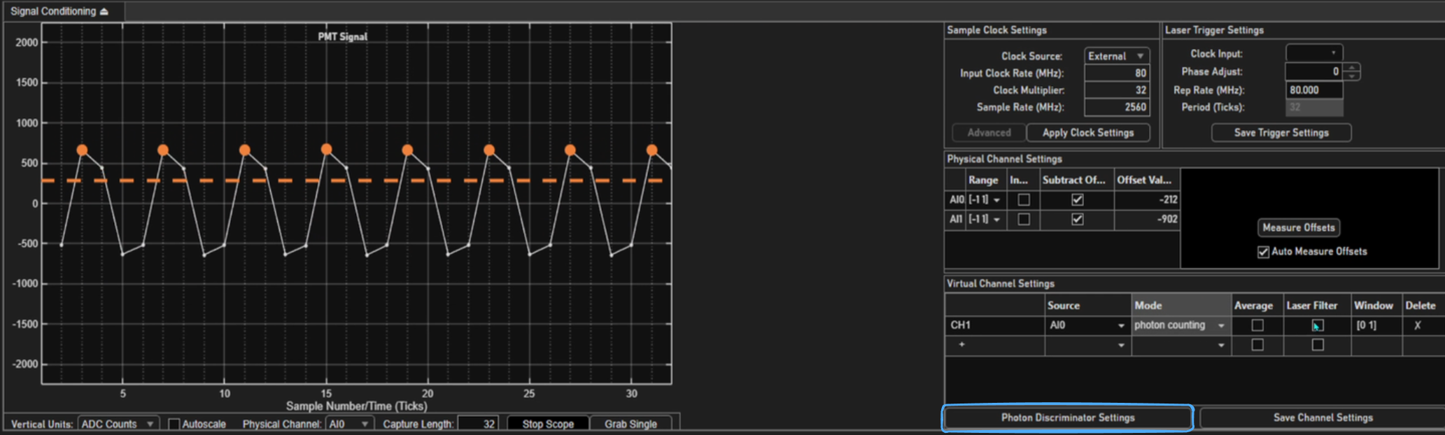
The threshold can also be set by typing in a value.
To do this, click the Photon Discriminator Settings button,
and edit the text in the box labeled Detection Threshold.
There is a second detection mode called Peak Detect. In this mode, a second plot is made from the original PMT signal called the Differentiated PMT Signal.
This plot is made by simply taking a sample’s value and subtracting the sample value from a previous sample.
The threshold is now applied to this differentiated PMT signal rather than the original.
The number of ticks separating these samples is known as the Differentiation Width, and is settable
from the Photon Discriminator Settings.
Virtual Channels
With Virtual channels, several channels worth of image data can be saved from a common high speed analog input port. For example, SI channels 1 and 2 can each display input collected from HSAI1. Virtual channel 1 could use a photo integration pipeline where as virtual channel 2 could use a photon counting pipeline for the same PMT data.
In CH1 under the Source column (row 1, column 2), one can specify that SI channel 1 should actually read the PMT signal from HSAI1 rather than HSAI0.
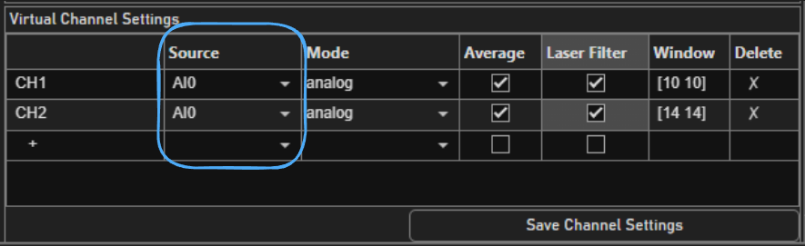
Up to 32 virtual channels can be added.
Virtual channels can be enabled to display or save from the Channels GUI in the left pane.
To remove virtual channels, select delete in the Source column for the row of the virtual channel that should be deleted.
Time Correlated Photon Counting
This feature is simply a combination of the photon counting feature and Temporal Demultiplexing.
If the sampling rate is synchronized with the laser rep rate, virtual channels can be used to bin samples by user defined temporal windows to separate out photons emitted by fluorophores with different fluorescent lifetimes. The windows are defined relative to each laser pulse.
First the external laser trigger must be configured. See the Sample Clock Settings. Set the Clock Source to External.
Then set the input clock rate to the external clock rate (which must be between 62.5MHz and 84.375MHz).
The Clock Multiplier must be 32; The resultant sampling rate should be between
2.0 and 2.7 GHz. In the laser trigger settings panel, set the Input Port in the Laser Trigger Settings panel to CLK IN.
Finally, click Apply Clock Settings.
Now acquire a number of samples from the signal scope greater than 4 times the number of samples collected between laser pulses, i.e. 4 * Clock Multiplier.
Verify that the laser clock frequency is measured correctly from the Laser Trigger Settings panel under Detected Freq (MHz).
The laser clock will now be overlayed on the PMT signal as dashed and solid red lines.
Between the dashed and solid red lines will be a number of ticks equal to
the Clock Multiplier. Windows can now be drawn over the PMT signal relative to the laser clock for each virtual channel.